/** \page multifit_3sfd Modeling of 3sfd with multifit
\tableofcontents
\section intro Introduction
In this example, MultiFit is used to build a model of porcine mitochondrial
respiratory complex II (PDB id 3sfd), using crystal structures of its
4 constituent proteins, a cryo-electron microscopy (EM) map of the entire
complex, and information from proteomics.
(See also \ref emagefit_3sfd for building models using 2D EM class averages
instead of 3D maps.)
All steps in the procedure use a command line tool called
multifit.py. For full help on this tool, run from a command line:
\code{.sh}
multifit.py help
\endcode
\section setup Setup
First, obtain the input files used in this example and put them in the
current directory, by typing:
\code{.sh}
cp /multifit/3sfd/* .
\endcode
(On a Windows machine, use 'copy' rather than 'cp'.) Here,
is the directory containing the IMP example files. The full path to the files
can be determined by running in a Python interpreter 'import IMP.multifit;
print IMP.multifit.get_example_path('3sfd')'.
The first step is to create an input file listing the subunits involved in the
complex. This file is a text file with a simple format; it simply contains one
line per component with the following information: the name that MultiFit will
use for the component, the name of the file containing the atomic coordinates,
and flag indicating whether placements of the subunit should be sampled locally
(0) or globally (1). The default for the fitting flag is 1 (global search).
If the user has prior knowledge or a good hypothesis as to the subunit
position, he or she can provide the proposed subunit placement in the atomic
coordinates file and ask for a local search.
In this case, no prior knowledge is assumed, and so the subunits file looks
like:
\verbatim
3sfdA 3sfd.A.pdb 1
3sfdB 3sfd.B.pdb 1
3sfdC 3sfd.C.pdb 1
3sfdD 3sfd.D.pdb 1
\endverbatim
This file is already provided, as 3sfd.subunits.txt.
The next step is to create two other input files that guide the MultiFit
protocol. This is done by using MultiFit's 'param' command, by running on a
command line:
\code{.sh}
multifit.py param -i 3sfd.asmb.input -- 3sfd.asmb 3sfd.subunits.txt 30 3sfd_15.mrc 15 3. 335 27.0 -6.0 21.0
\endcode
The 'param' command takes as arguments the coarseness level in residues (30),
the resolution of the map in angstroms (15), the map spacing in angstroms (3),
the density threshold (335), and the origin of the map in angstroms
(27.0, -6.0, 21.0). The spacing (or pixel size) and origin are often stored
in the map header. To view the map header, run:
\code{.sh}
view_density_header.py 3sfd_15.mrc
\endcode
The resolution is typically not stored in the map header; it is usually
provided in the corresponding publication and can also be found in the
corresponding \external{http://www.ebi.ac.uk/pdbe/emdb/,EMDB} entry.
A threshold is often provided by the author in the EMDB entry as
"Recommended counter level" under the "Map Information" section.
Alternatively, IMP provides a utility to calculate an approximate counter
level based on the molecular mass of the complex, which can be run as:
\code{.sh}
estimate_threshold_from_molecular_mass.py 3sfd_15.mrc 1092
\endcode
The first file generated by MultiFit, 3sfd.asmb.input, provides
information on each of the subunits and their assembly density map, such as
names of the files from which the input structures and map will be read,
and those to which outputs from later steps will be written. The second file,
3sfd.asmb.alignment.param, specifies scoring and optimization
parameters for each step of the MultiFit protocol. These parameters can be
adjusted if necessary to handle difficult modeling cases.
(Note that two other files are also created, with a .refined extension.
These can be used for model refinement, which is discussed later.)
\section anchors Create the assembly anchor graph
Next, a reduced representation of the assembly density map is generated
using the Gaussian Mixture Model, by running:
\code{.sh}
multifit.py anchors 3sfd.asmb.input 3sfd.asmb.anchors
\endcode
This command computes a reduced representation of the EM map that best
reproduces the configuration of all voxels with density above the density
threshold (provided in the 3sfd.asmb.input file) as a set of
3D Gaussian functions. (The default number of Gaussians is the number of
components. However, if the sizes of the subunits differ, it is recommended
to use the -s option to set the number of residues encapsulated in
each Gaussian. For example, with 50 residues per Gaussian, a 170-residue
protein should use 3 Gaussians and a 260-residue protein should use
5 Gaussians.) The reduced representation is written out as a PDB file
containing fake CA atoms, where each CA corresponds to a single anchor point,
and also as a \external{http://www.cgl.ucsf.edu/chimera/,Chimera} cmm file.
\section fit_fft Fit each protein to the map
First, fit each protein to the map using a FFT search either globally or
locally:
\code{.sh}
multifit.py fit_fft -a 30 -n 1000 -v 60 -c 6 3sfd.asmb.input
\endcode
The output is a set of candidate fits. In each file, a single subunit is
rigidly rotated and translated to fit into the density map. Each fit is
written out as the transformation (rotation and translation) required to
place the original subunit in the density map. The fitting of a subunit
into the density map is performed by globally searching for subunit
transformations yielding high cross-correlation between the subunit and
the map via a fast Fourier transform.
Next, a list of valid fit indexes is created. As below, this list is
simply the top 3 hits from fit_fft, but they could be filtered by other
criteria (e.g., proximity to anchor points) if desired. Note that the more fit
indexes used, the longer it will take to combine the fits into a global solution
in further steps in the protocol (but the more likely it is that the optimum
solution is found). For a quick demonstration, the 3 top fits are sufficient,
but 10 or more fits are recommended in most cases. Do this by running:
\code{.sh}
multifit.py indexes 3sfd 3sfd.asmb.input 3 3sfd.indexes.mapping.input
\endcode
\section proteomics Create a proteomics restraint file
Here, the restraint file used in the next assembly step is created.
This file instructs MultiFit how to combine the individual subunit fits
created above into a global solution of all subunits simultaneously fitted
into the map. First, MultiFit can generate a basic proteomics file, indicating
between which pairs of proteins a complementarity restraint (i.e., that the
surfaces of the proteins should fit and complement each other) should
be calculated:
\code{.sh}
multifit.py proteomics 3sfd.asmb.input 3sfd.asmb.anchors.txt 3sfd.asmb.proteomics
\endcode
The user can then add additional information from proteomics experiments to
this file. Here, 7 simulated residue-residue cross-link restraints are added.
The excluded volume (EV) pairs are also updated to calculate complementarity
restraints between pairs of proteins as indicated by the cross-link
restraints. After these additions, the final 3sfd.asmb.proteomics
file looks like:
\verbatim
|proteins|
|3sfdA|1|613|nn|nn|
|3sfdB|1|239|nn|nn|
|3sfdC|1|138|nn|nn|
|3sfdD|1|102|nn|nn|
|interactions|
|residue-xlink|
|1|3sfdB|23|3sfdA|456|30|
|1|3sfdB|241|3sfdC|112|30|
|1|3sfdB|205|3sfdD|37|30|
|1|3sfdB|177|3sfdD|99|30|
|1|3sfdC|95|3sfdD|132|30|
|1|3sfdC|9|3sfdD|37|30|
|1|3sfdC|78|3sfdD|128|30|
|ev-pairs|
|3sfdB|3sfdA|
|3sfdB|3sfdC|
|3sfdC|3sfdD|
\endverbatim
This modified file is already present, as 3sfd.xlinks.proteomics.
Replace the basic file with it by running:
\code{.sh}
cp 3sfd.xlinks.proteomics 3sfd.asmb.proteomics
\endcode
Note that these restraints will be used to create DOMINO’s junction tree.
DOMINO works most efficiently if the size of the intermediate subsets is small.
Use the multifit.py merge_tree command to view the tree defined
by the restraints. To reduce the size of the subsets, the user can determine
which restraints are used to define the merge tree by setting the first
value in the xlink definition. Setting the value to 0 instead of the default 1
specifies that the restraint is evaluated only at the root of the tree
and not in an intermediate merging step.
\section assemble Assemble subunits
The fits are combined into a set of the best-scoring global configurations
by running:
\code{.sh}
multifit.py align 3sfd.asmb.input 3sfd.asmb.proteomics 3sfd.indexes.mapping.input 3sfd.asmb.alignment.param 3sfd.asmb.combinations 3sfd.asmb.combinations.fit.scores
\endcode
The output is the file 3sfd.asmb.combinations which contains a ranked
list of combinations (best scored first). Each combination is simply a list of
4 numbers, where the first number is the index of the fit for the first subunit,
the second number the fit for the second subunit, and so on.
The scoring function used to assess each fit includes the quality-of-fit
of each subunit in the map, the protrusion of each subunit out of the map
envelope, the shape complementarity between subunits, as indicated in the
proteomics file, and distance restraints as defined by proteomics data,
also from the proteomics file. The optimization avoids exhaustive enumeration
of all possible mappings of subunits to anchor points by means of a
branch-and-bound algorithm combined with the DOMINO divide-and-conquer
message-passing optimizer using a discrete sampling space.
\section visualization Visualization
Finally, models can be generated as PDB files from the fits and best
combinations by running:
\code{.sh}
multifit.py models -m 5 3sfd.asmb.input 3sfd.asmb.proteomics 3sfd.indexes.mapping.input 3sfd.asmb.combinations model
\endcode
This generates PDB files for the 5 best-scoring solutions, calling them
model.0.pdb, model.1.pdb, and so on.
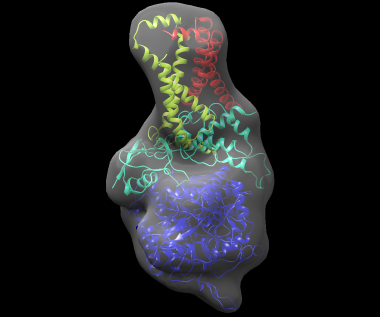
The best-scoring solution, shown fitted in the density map of the complex,
is shown below:
 \section analysis Analysis
If a reference structure for each subunit is available, the 'reference'
command can be used to compare the models to the reference. To use this command,
modify 3sfd.asmb.input and add the filename of each reference subunit
structure in the rightmost column. In fact, the input subunit structures are
already in their native conformation, so these structures can be used. The
file 3sfd.asmb.input.ref already has this modification. Then run:
\code{.sh}
multifit.py reference -m 5 3sfd.asmb.input.ref 3sfd.asmb.proteomics 3sfd.indexes.mapping.input 3sfd.asmb.combinations
\endcode
This will report, for the top 5 combinations, the all-atom RMSD between the
model and the reference structure of the complex, and a list of placement
scores, one for each subunit. Each placement score is the distance that the
subunit must be moved to reach the reference structure and the angle through
which it must be rotated.
*/
\section analysis Analysis
If a reference structure for each subunit is available, the 'reference'
command can be used to compare the models to the reference. To use this command,
modify 3sfd.asmb.input and add the filename of each reference subunit
structure in the rightmost column. In fact, the input subunit structures are
already in their native conformation, so these structures can be used. The
file 3sfd.asmb.input.ref already has this modification. Then run:
\code{.sh}
multifit.py reference -m 5 3sfd.asmb.input.ref 3sfd.asmb.proteomics 3sfd.indexes.mapping.input 3sfd.asmb.combinations
\endcode
This will report, for the top 5 combinations, the all-atom RMSD between the
model and the reference structure of the complex, and a list of placement
scores, one for each subunit. Each placement score is the distance that the
subunit must be moved to reach the reference structure and the angle through
which it must be rotated.
*/